

MAY 10, 2021
Law of Conservation of Ca (Rational Method version)
Tom Walski, Ph.D, P.E, Industry Analyst and Bentley Fellow
Key Takeaways
- The Law of Conservation of Mass Exception: While physical mass is conserved, peak flows calculated using the Rational Method cannot be simply added together to find cumulative downstream peak flows.
- The Impact of Travel/System Time: Peak rainfall intensity decreases as duration increases (Intensity-Duration-Frequency curve relationship). As water travels further downstream, the cumulative system time increases, which lowers the corresponding peak rainfall intensity used for calculations.
- Attenuation in Calculations: Due to peak flow attenuation, the calculated peak flow of a combined downstream channel is less than the raw mathematical sum of its parts (e.g., 30 cfs + 36 cfs = 53.2 cfs instead of 66 cfs).
- Novice Misconceptions: This standard hydrological variance frequently confuses beginner hydraulic modelers using tools like Bentley OpenFlows StormCAD, OpenRoads Designer, CivilStorm, and SewerGEMS.
We all know that as two flows meet, according to the Law of Conservation of Mass, the resulting flow will be the sum of the two flows.
We saw last week that that rule doesn't apply when you're summing up peak flows for premise plumbing using fixture units. This week we'll see another example that defies the Law of Conservation of Mass. This time, the exception comes about in the context of stormwater, when we add the peak flows from catchments using the Rational Method.
This issue shows up when the peak flow from one catchment is, for example, 3 cfs, and the flow from the next catchment is 2 cfs, and the total flow is less than 5 cfs. To determine why this happens, let's look at the Rational Method, which was developed by Mulvaney in the British Isles in 1851. It is described by:
Q = Cia (1)
Where:
- Q = flow (cfs)
- C = runoff coefficient
- i = peak rainfall intensity (in/hr)
- a = drainage area (acres)
A logical person (we won't call them rational) should be able to simply sum the flows from two catchments as shown below:
Q = C1*i1*a1 + C2*i2*a2 (2)
But that equation doesn't work because the peak is attenuated. As one moves farther downstream, the time over which the peak intensity increases and hence, the flow calculated decreases. The 15-minute peak intensity is greater than the 30-minute peak intensity. This gets into intensity, duration, frequency (idf) relationships which can be given as equations or tables for any areas with sufficient records. As the water moves downstream, the duration for the flow to reach any point increases, and the intensity corresponding to that duration decreases. A typical intensity duration curve for a given frequency showing the inverse relationship between intensity and duration can be written as:
i = d / (b + D)^n (3)
Where:
- D = duration (min)
- b, d, n = coefficients
Therefore, equation (2) must be replaced by:
Q = i (C1*a1 + C2*a2) (4)
Where the intensity in equation (4) is the intensity of the overall upstream catchments based on the system time of the longest path, which includes both the time of concentration in the catchment and the travel time in conduits (i.e. pipes and channels).
This is best illustrated by an example. Consider the stormwater system shown below:
Figure 1: Stormwater System Diagram I
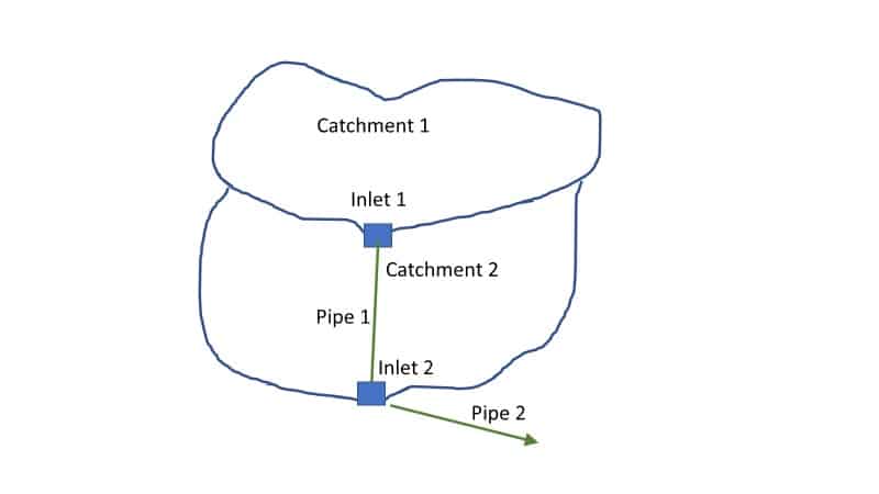
The calculation of flow is shown in the table below. If the flows were added to determine the flow in Pipe 2, the result would be 66 cfs. But because the peak upstream intensity decreases by moving downstream, the flow is only 53.2 cfs as shown below. The travel time for Pipe 1 must be added to the time of concentration for Catchment 1 to determine the system time as the peak flow approaches Inlet 2. This travel time is usually small but not insignificant compared with the time of concentration of the upstream catchment. (The value for system time at the downstream end of Pipe 2 is 25 + 3 for the travel time in Pipe 2.)
Figure 2: Flow Calculation Table

Figure 3: Stormwater System Diagram II
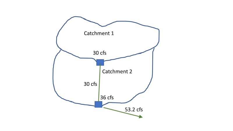
Such results tend to trouble novice users of the Rational Method as applied in Bentley's OpenFlows StormCAD, OpenRoads Designer, or if the user selects the GVF-Rational Solver in Open Flows CivilStorm and OpenFlows SewerGEMS. They tend to have the idea that 30 + 36 = 66. But as shown with fixture unit methods, combining peak flows is not the same as adding flows.
To learn more about drainage calculations, get a copy of Bentley's Stormwater Conveyance Modeling and Design which explains the background for these calculations. We also have a few Bentley Communities wiki articles that discuss this topic further: